Assignment 03: Mapping Overlaps Intersections and Paths

Due: October 21, 2020

Assignment 03 Deliverables

To receive credit and feedback on this project please upload the following to canvas by 10/28

1. Answers to the following questions in a .txt file:

   1. Which Newark park has the greatest number of schools within 1/4 mile of its boundary?
   2. How many people live within walking distance of a park? And what percentage of Newark’s total population is this? (using select by location method)
   3. What is the total 2010 population of Newark according to this dataset?
   4. What are the units of the tot_area field you calculated?
   5. How many people live within walking distance of a park? And what percentage of Newark’s total population is this? (using proportional split estimation)

2. A copy of this PDF of geoprocessing diagrams that you have annotated in response to each question. Please complete this portion of the assignment last. Detailed instructions are included at the bottom of this page. (Note you must be logged in to your NJIT email to access)

File names for you .txt file and annotated PDF should follow this naming convention exactly: lastname_firstname_assignment01

Access to parks

In this assignment you will answer two spatial research questions about access to parks in Newark:

• Which park has the greatest number of schools within 1/4 mile? (i.e. which park serves the greatest number of schools?)
• What percentage of Newark’s population lives within walking distance of a park? Where walking distance is defined as within 1/4 mile of the perimeter of any park.

Datasets used (download all here):

• Newark Parks
• Newark schools
• Population by census block in 2010

Geoprocessing

In order to answer these research questions you will use a new set of methods: geoprocessing. Maantay & Zeigler (2006) Chapter 9 introduces the core concepts we will be working with here. Make sure you’ve closely read the excerpted portion of that chapter (esp pp 213-2018) before going any further in this assignment.

“Geoprocessing is the general term given to a variety of operations on spatial data in which data layers are combined in different ways to yield new spatial or attribute information” (Maantay & Zeigler 213).

Geoprocessing relies/takes advantage of the core abstraction in GIS: describing phenomena through a series of discrete data layers.

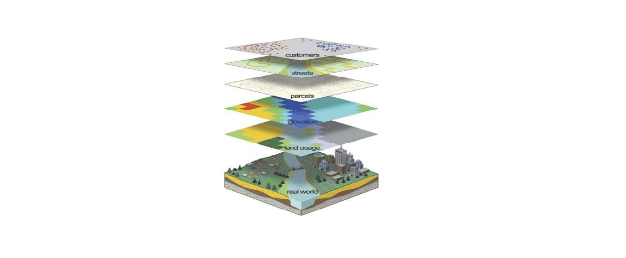
Geoprocessing operations are a set of methods to study spatial relationships within and between data layers. The primary spatial relationships that are studied are:

• Proximity
• Contiguity
• Connectivity
• Containment

All spatial data has both geometric/geographic information (its shape, size, position) as well as attribute information (values in its attribute table in the case of vector data, and the value for each cell in raster data).

Geoprocessing operations primarily manipulate the geometric/geographic relationships between layers however, they also produce a change in the attribute information. Understanding the relationship between changes in geometry and the associated impact on the attribute table of the layer involved is central to understanding how to use geoprocessing operations to uncover previously invisible information and relationships between data layers.

In this exercise we will use geoprocessing operations to answer a series of questions about access to parks in Newark.

Along the way you will be asked to reason through how a number of operations work conceptually through a series of diagrams.

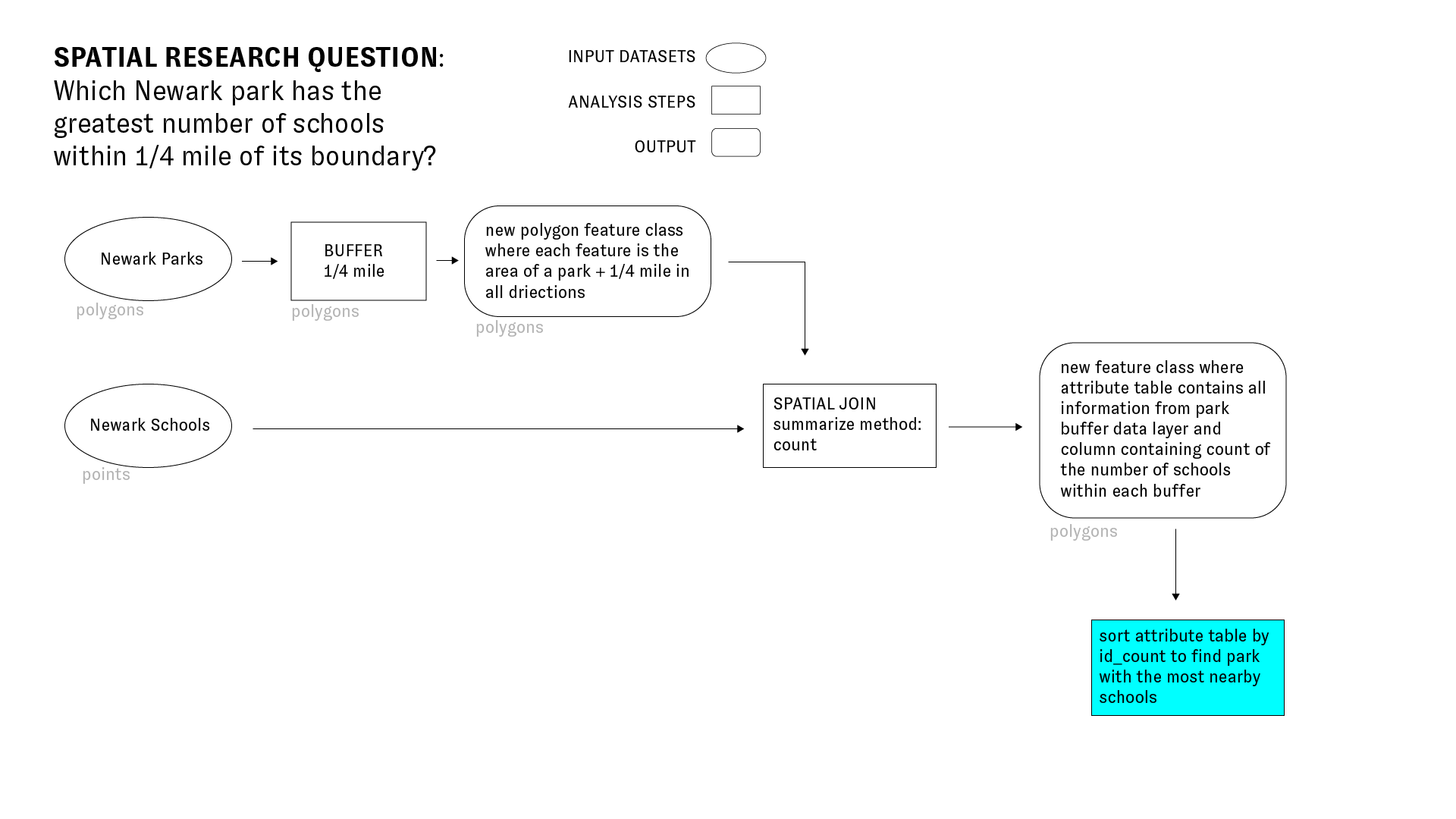
Which Newark park has the greatest number of schools within 1/4 mile of its boundary?

To answer the question above we will use two key geoprocessing methods: by creating buffers around Newark Parks and performing a spatial join between those buffers and Newark Schools to see how many schools fall within 1/4 mile of a park. The diagram below illustrates the methodology we will use to answer this question:

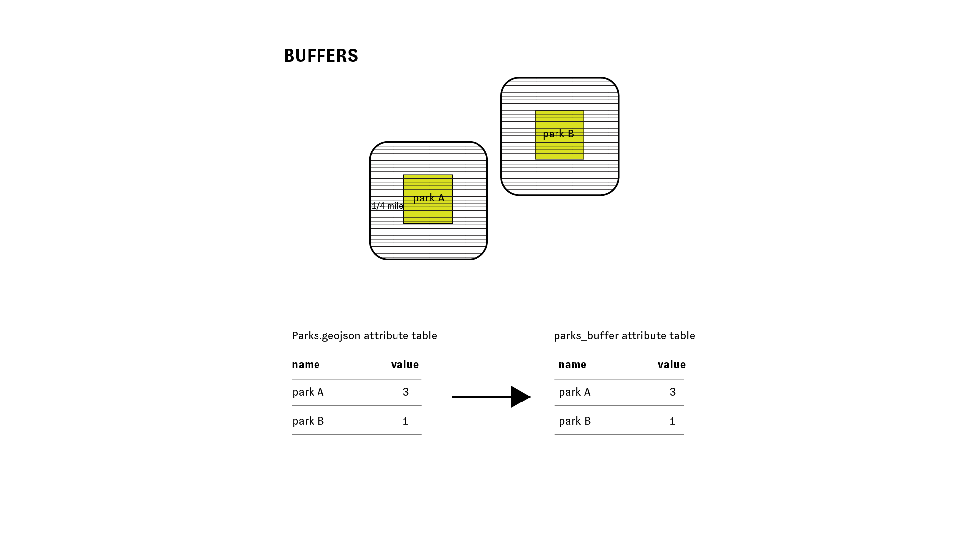
Buffers

Please see Maantay & Zeigler p. 215 for an introductory description of buffers.

This method is a form of analysis that allows us to measure spatial relationships of proximity.

The diagram below illustrates the relationship between the attribute table for the input features, and the attribute table for the new feature class which is produced after running the buffer tool.

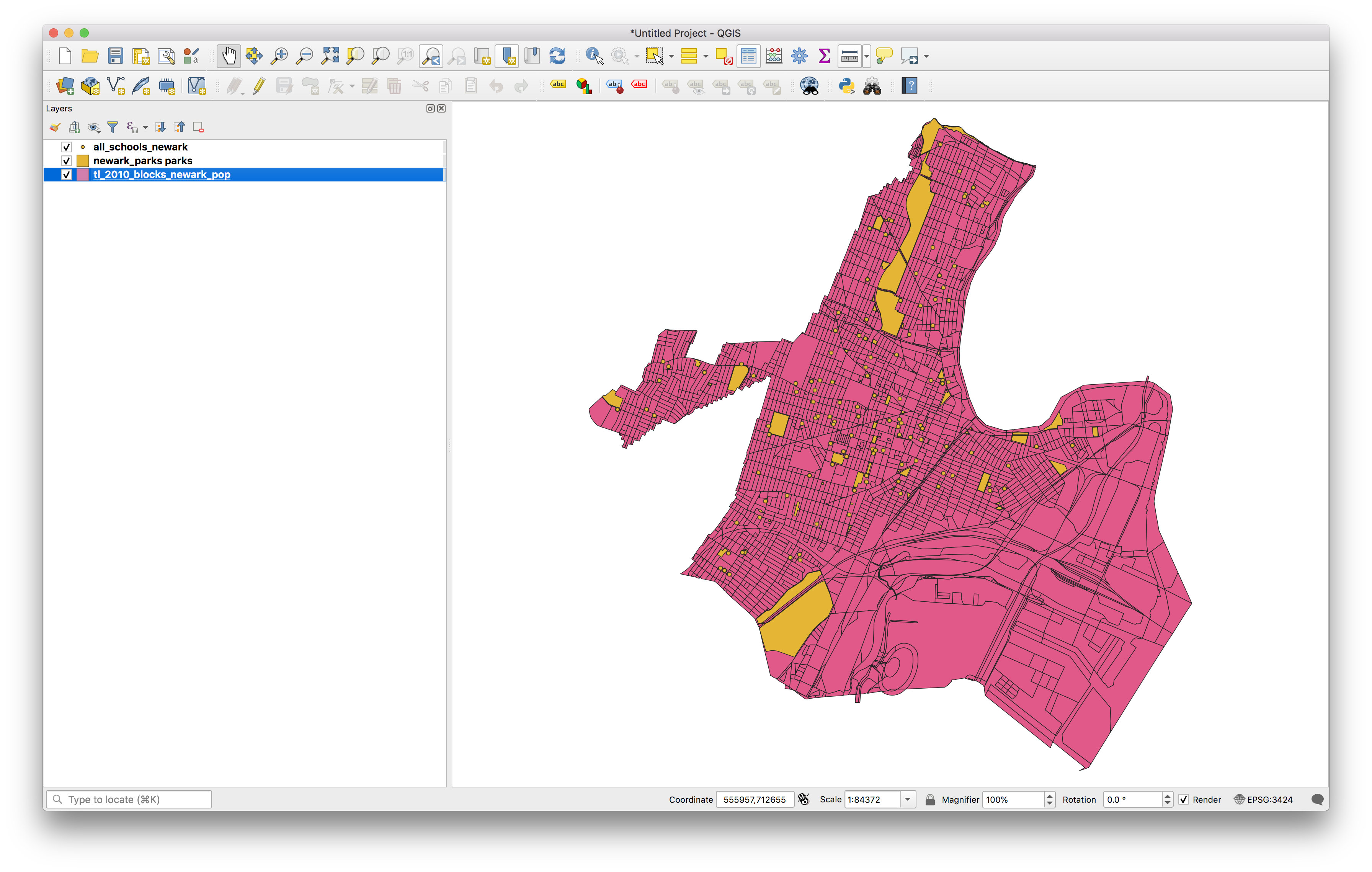
Open QGIS.

Add the datasets for this assignment which you can download here

Select from the top menu vector>geoprocessing tools>buffer and then make the following selections in the buffer dialogue box to create 1/4 mile buffers around each Newark Park:

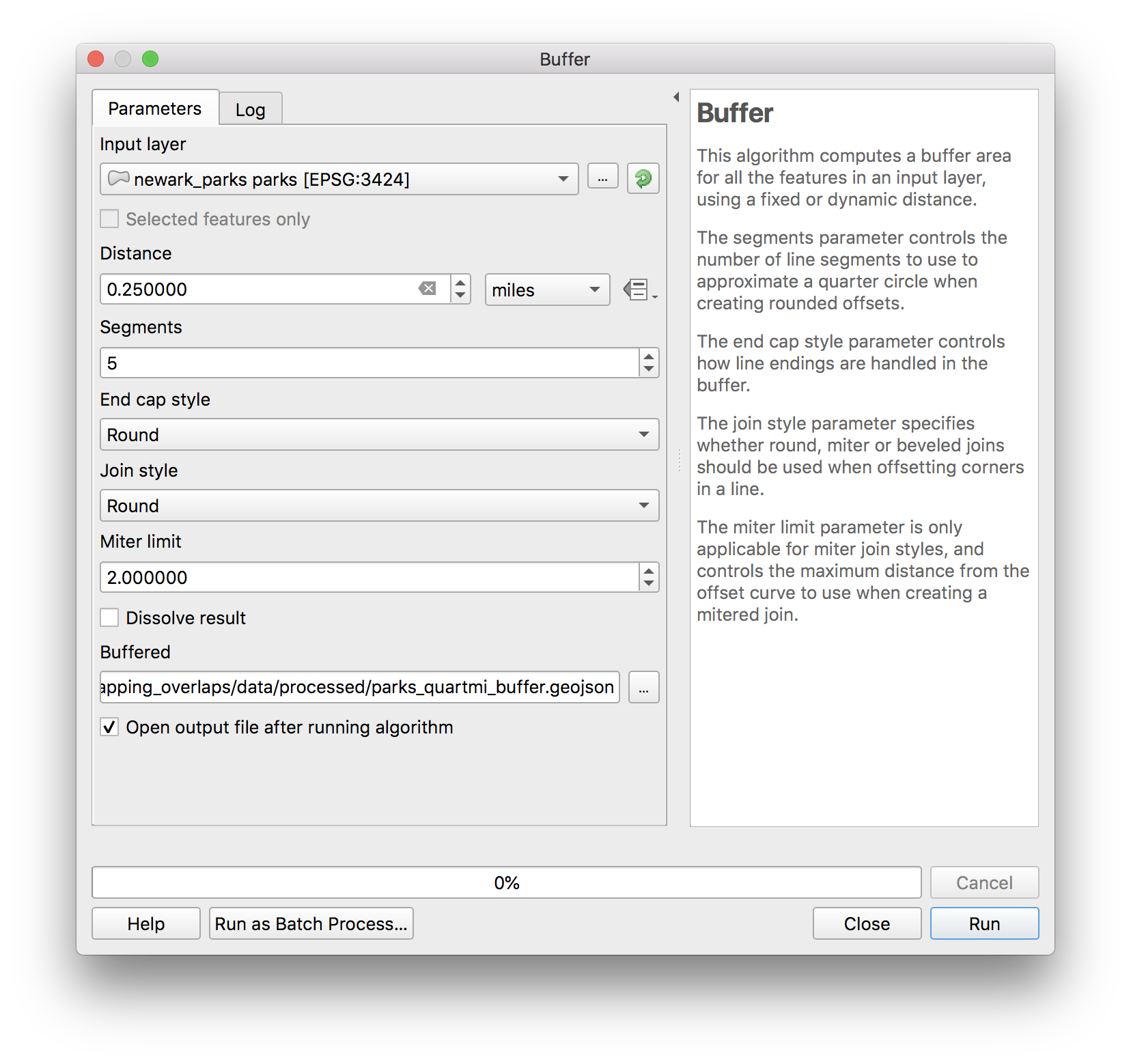
Create anew folder called process within the data folder for this assignment. Save the results as parks_quartmi_buffer.geojson. Click Run.

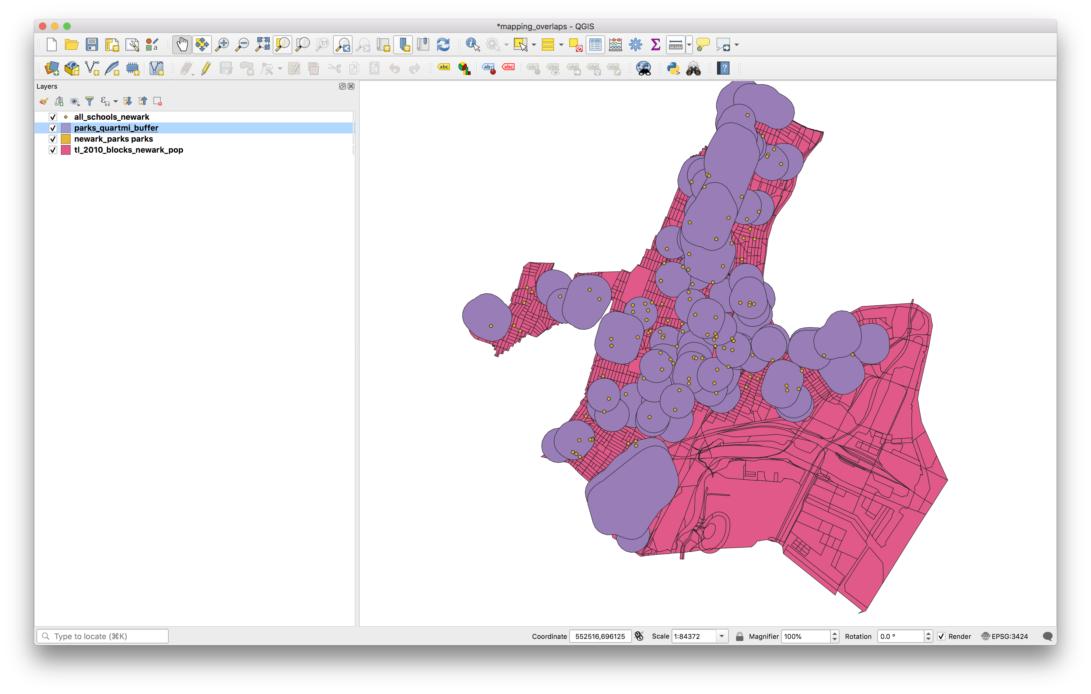
You should now see a new polygon feature class added to you map which is buffers of 1/4 mile around each park.

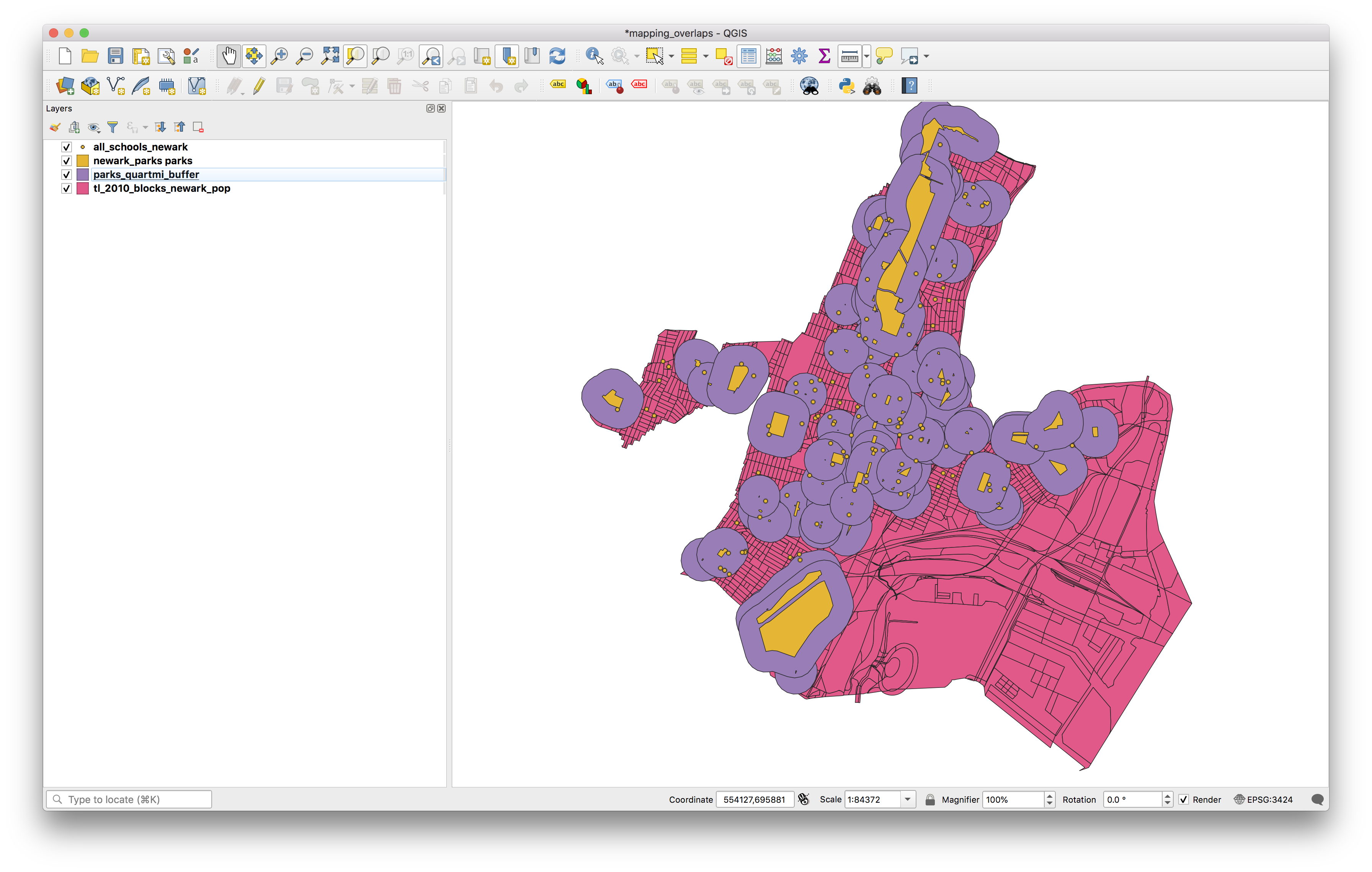
If you adjust the layer order to move the parks layer above the buffers you can see the relationship between each park and each buffer:

Spatial Join

Now we have successfully created a new dataset which shows us the areas that are within 1/4 mile of each park in Newark (including the park itself).

To answer our spatial research question Which Newark park has the greatest number of schools within 1/4 mile of its boundary? we now need to identify which schools fall within these buffers.

To do this we will perform a spatial join. For a conceptual introduction please re-read Maantay & Zeigler p. 218.

In a spatial join we are using the geometric and geographic relationships between two data layers to associate attribute information from one dataset with the attribute table for the other. In a spatial join, just as in a table join, the order matters and will impact the results of the spatial join.

Using our two input datasets as an example, joining the park buffers to the schools would yield the following results (shown as a diagram below):

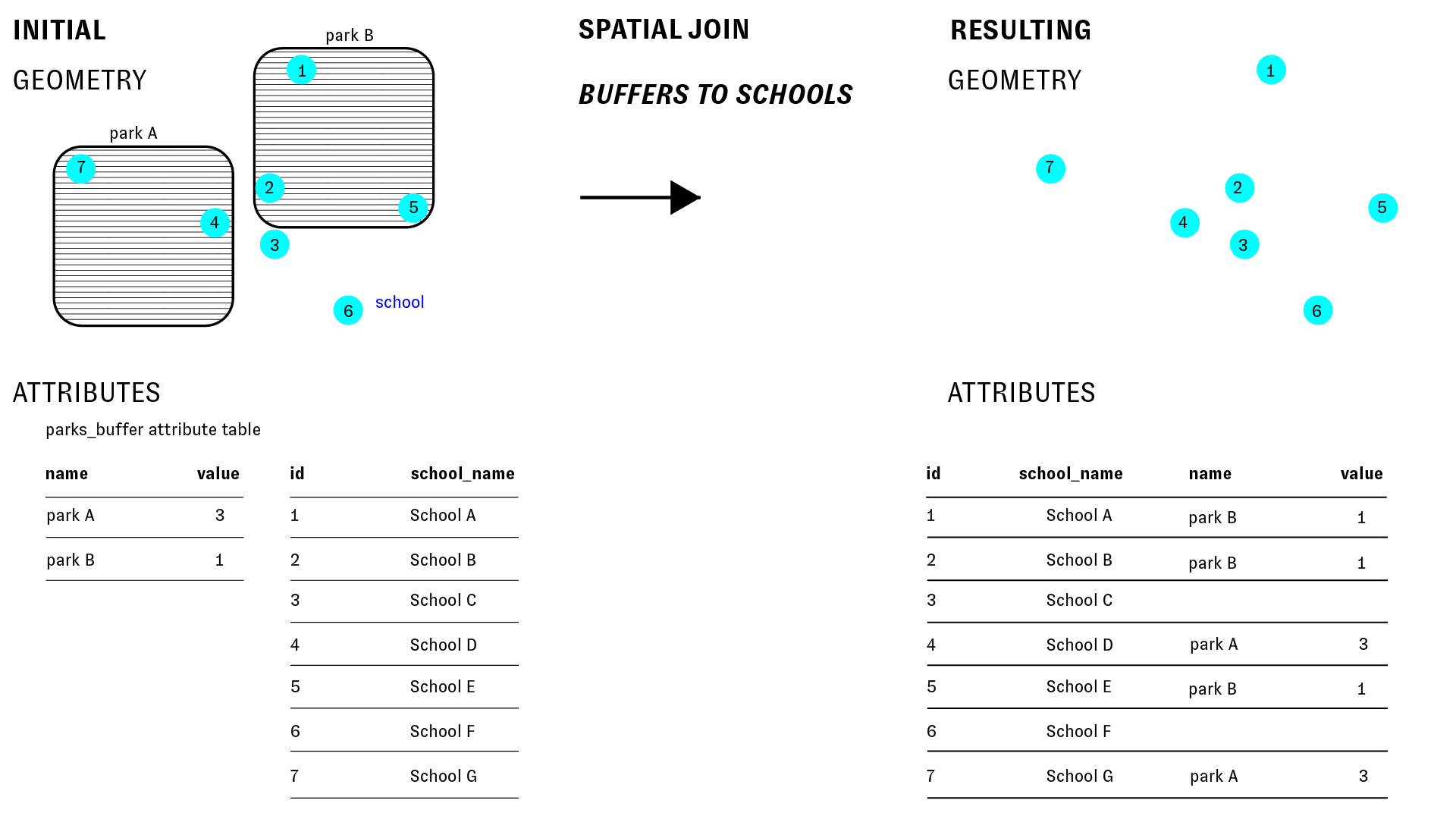
In the above example the schools are the input layer, and the park buffers are the join layer.

The resulting feature class has the same geometry of the school points, and its attribute table contains everything from the school points layer, with additional fields from the park buffers added.

What about the inverse: if we join the schools to the park buffers?

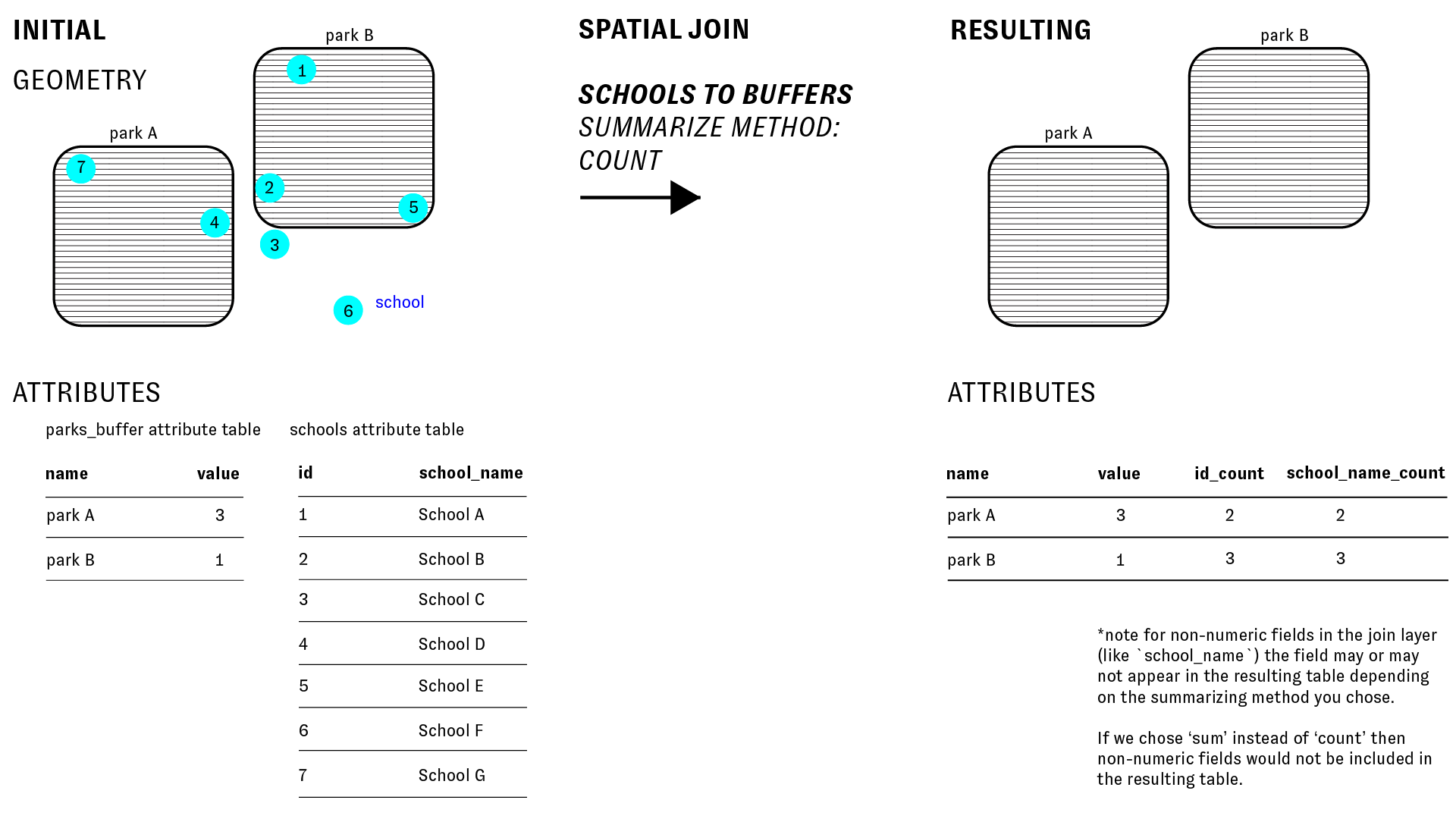
In this scenario, as the diagram below illustrates, there are multiple schools within each park buffer. Each park buffer is a single feature and corresponds with exactly one row in its attribute table. So in order to join information about multiple schools to each buffer we must summarize that information. We could take the count, sum, mean, max, first value, last value or other standard summary method.

The research question we are trying to answer right now is: Which Newark park has the greatest number of schools within 1/4 mile of its boundary? And to answer this we currently need to learn how many schools are within 1/4 mile of each park. Thus we want to take the count of the schools when we perform the spatial join.

The diagram below illustrates this and the impact of the spatial join on the attribute table:

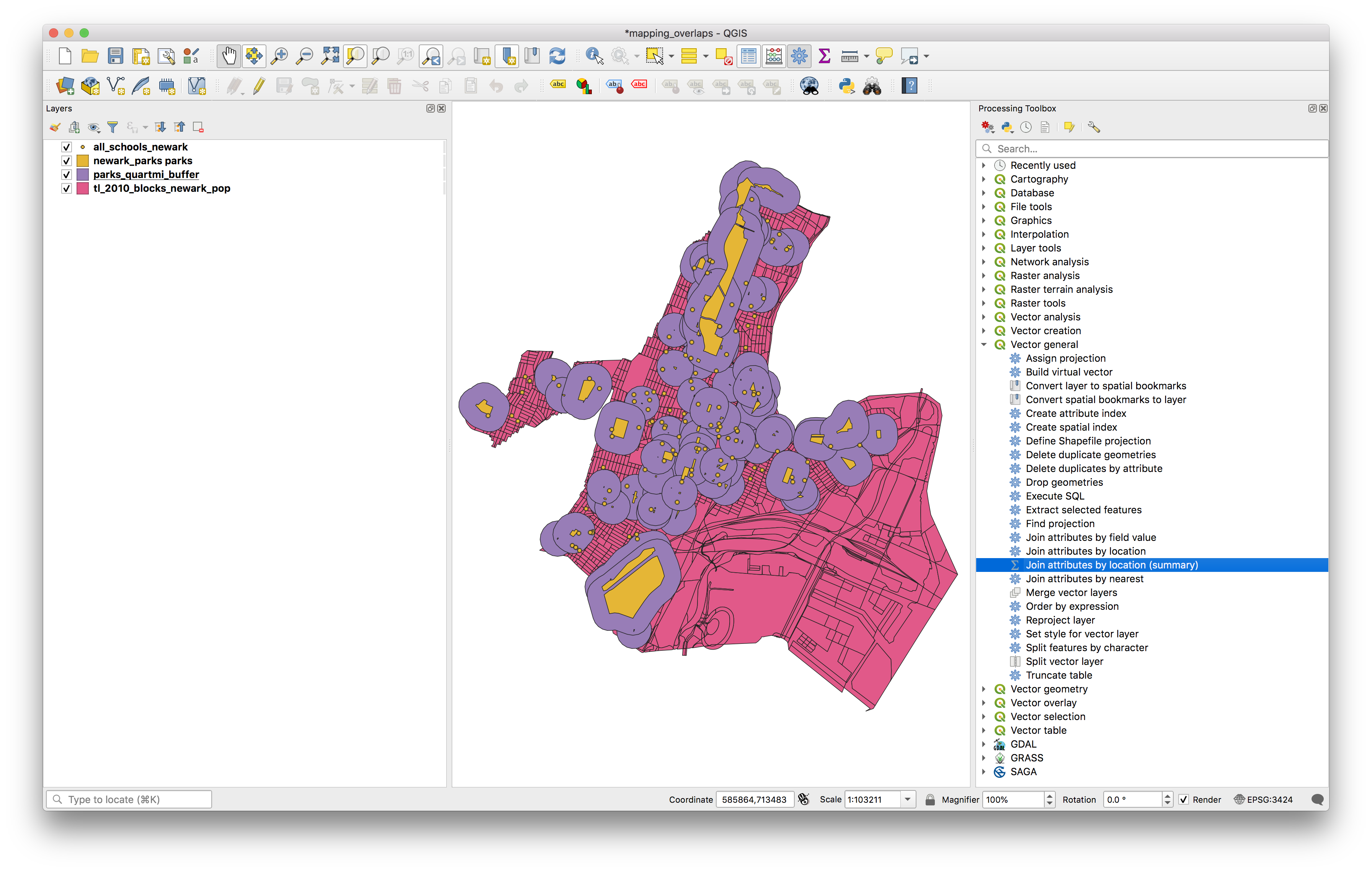
To do this in QGIS, open the Processing toolbox by selecting from the top menu Processing>Toolbox. When the toolbox opens expand the Vector general menu, and select Join attributes by location (summary). Notice that there is also a Join attributes by location tool, if performing a spatial join where each input feature corresponds with only one join feature (i.e. you do not need to summarize the join features) then use this tool.

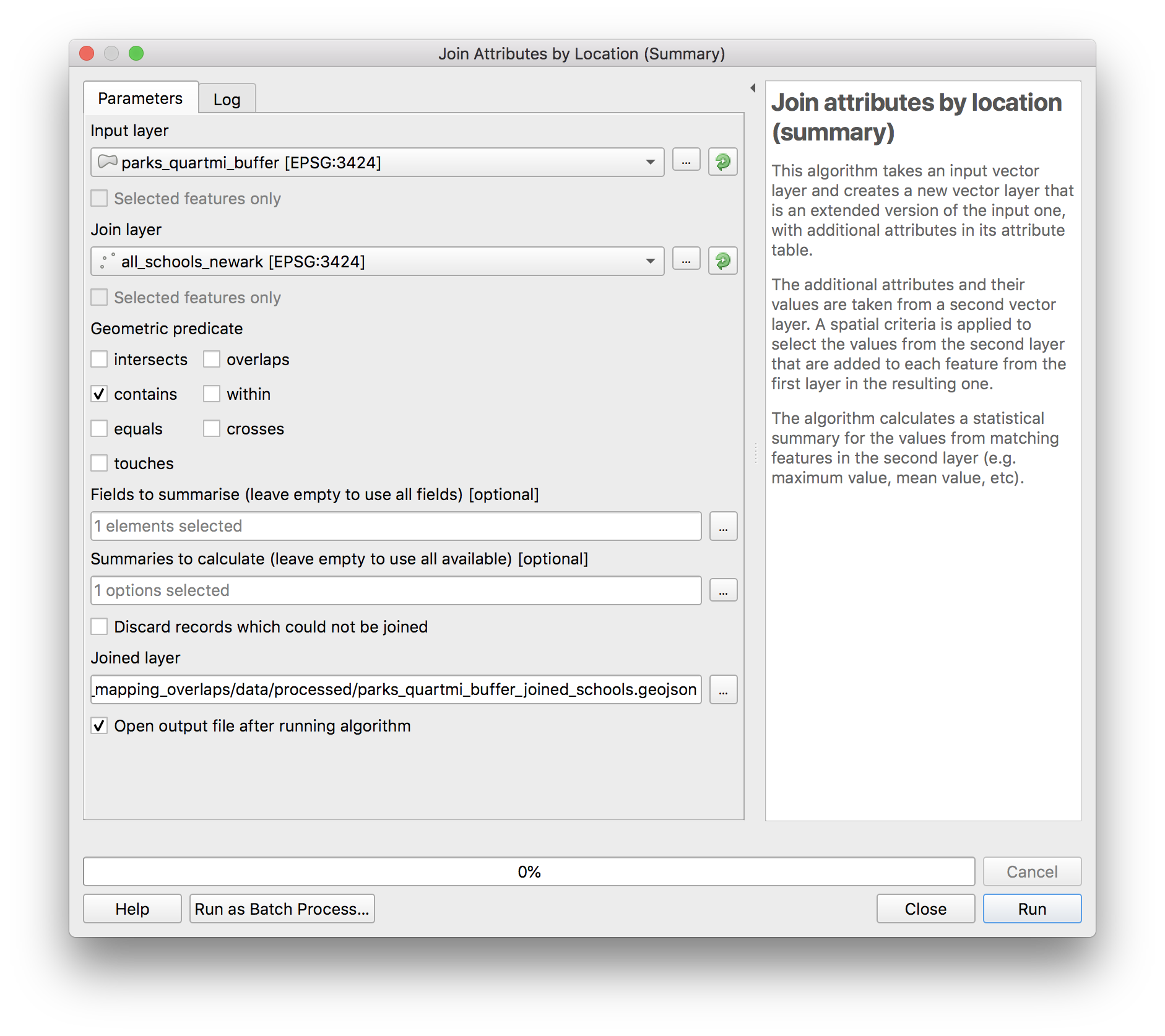
In the dialog box which opens make the following selections:

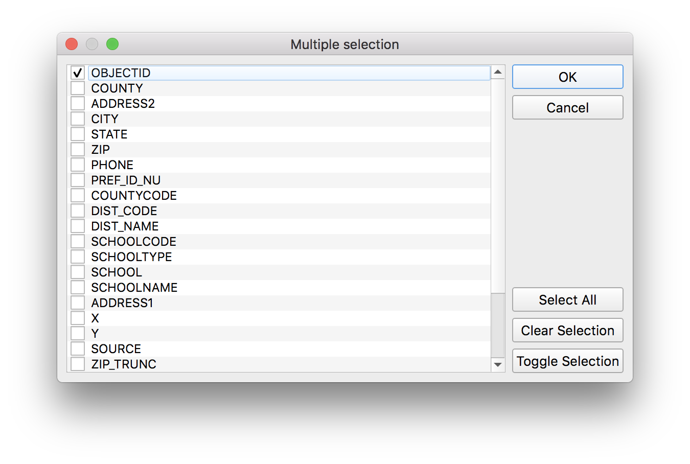
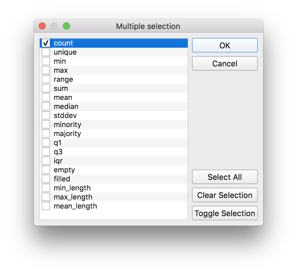
For the fields to summarize click on the button with ... to select the following:

And for the summaries to calculate click on the button with ... to select the following:

Save the new feature class in the process folder you created within the data folder for this assignment. Name the file parks_quartmi_buffer_joined_schools.geojson.

Click Run.

The resulting layer should be added to the layers panel on your map. Open the attribute table for parks_quartmi_buffer_joined_schools. Sort by the OBJECTID_count field by clicking on the name of that field in the attribute table. Which Newark park has the greatest number of schools within 1/4 mile of its boundary?

Supply this answer with your deliverables for this assignment.

What percentage of Newark’s population lives within walking distance of a park?

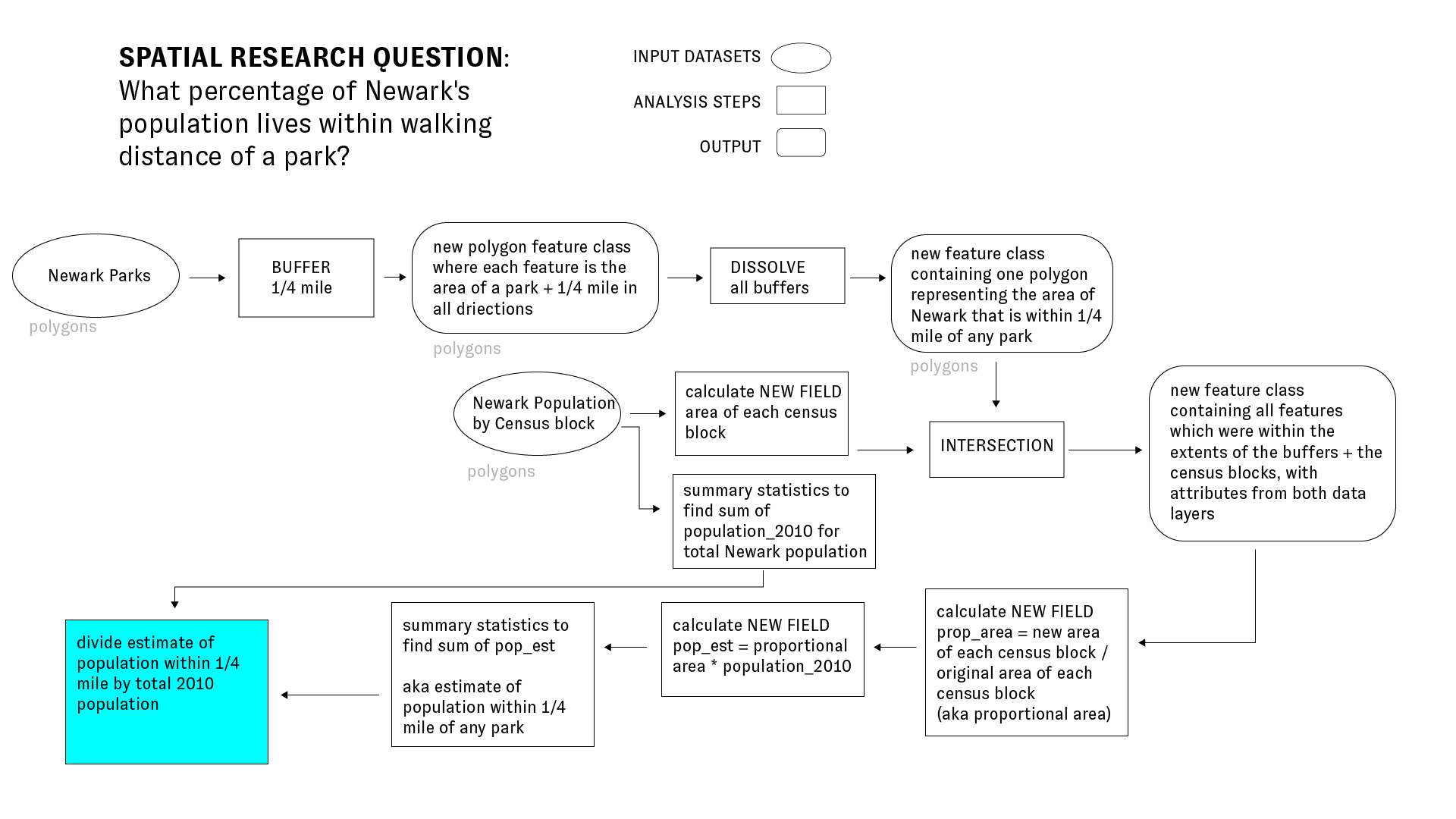
We’ll now work to answer a slightly more complicated question about access to parks in Newark. What percentage of Newark’s population lives within walking distance of a park? (Where walking distance is defined as within 1/4 mile of the perimeter of any park.)

Estimating the population within this area is a non-trivial problem. We have data about population however the finest geographic scale that this is released at is the Census block. And Census blocks do not align exactly with the areas within 1/4 mile of each park.

So we will need to develop a method for estimating, for the proposes of instruction we will compare two different methods. First by selecting all of the census blocks which intersect with a buffer for a park we will obtain a very coarse estimate. And then we will refine this using a technique called proportional split estimation.

Estimating population with select by location

In the first estimation method we will overestimate the total population by selecting all of those census blocks which intersect or are within the 1/4 mile buffers around each park. And we will consider the total population living within those census blocks as the estimated population. This is illustrated in the diagram below:

In QGIS open Vector > Research Tools > Select by location. Make the following selections:

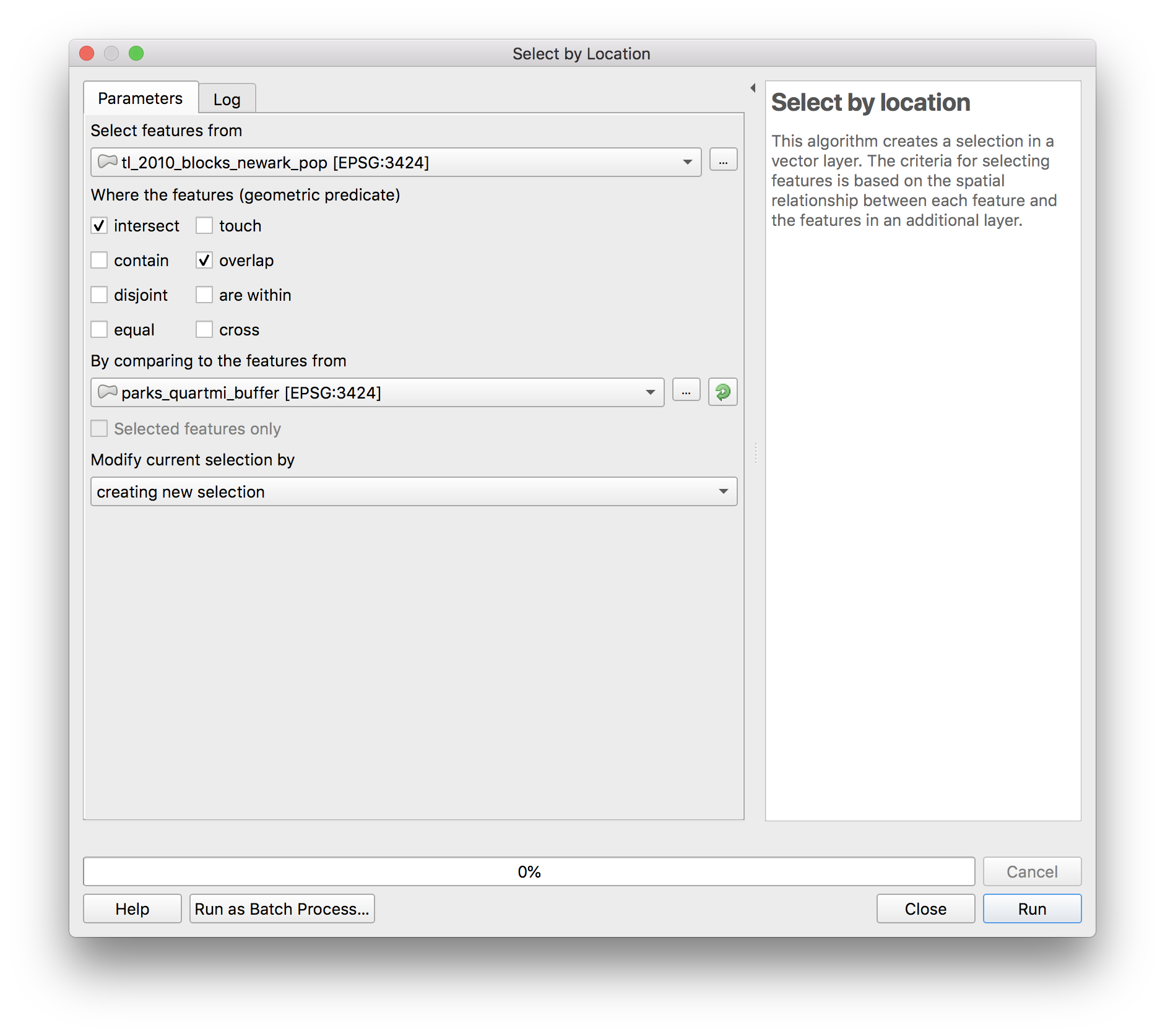
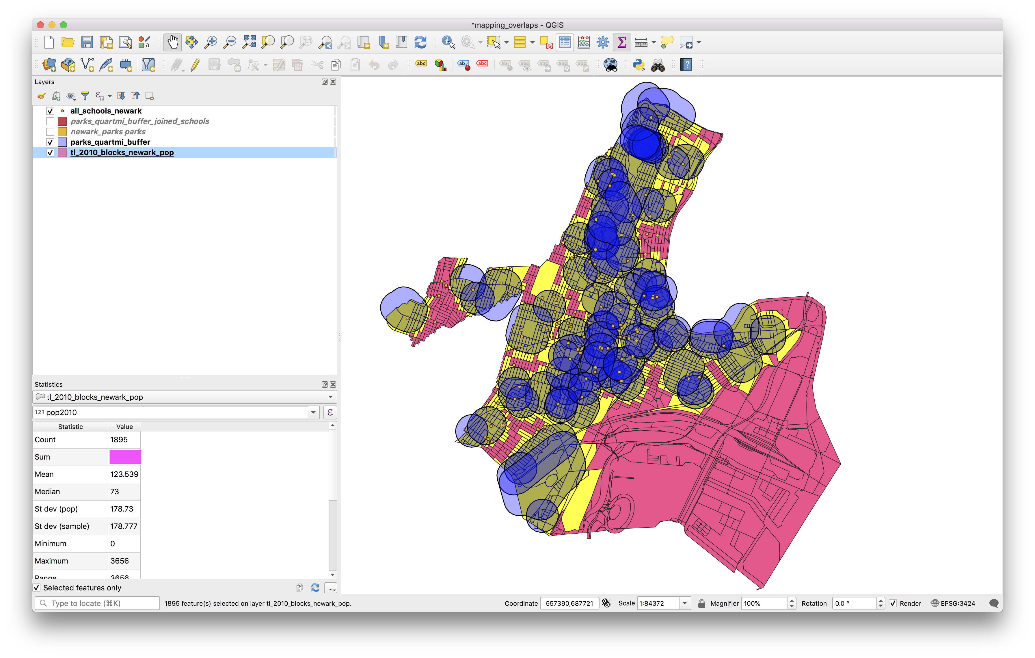
The results should look something like this (we’ve given transparency to the park buffers so it is easier to see the selected blocks below). Now to get summary statistics for the census blocks that were selected click the show summary statistic button (circled below).

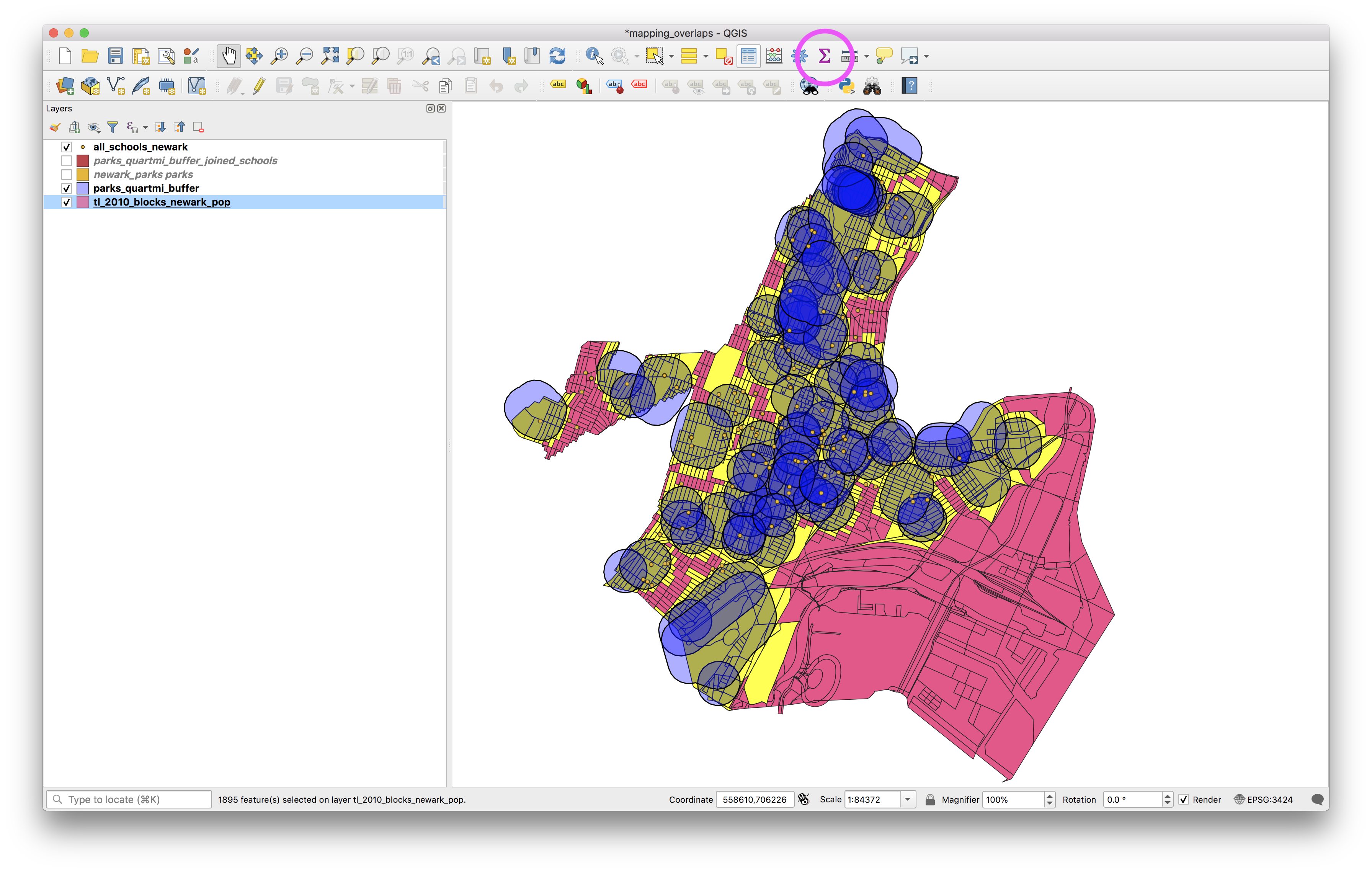
In the dialogue window that opens select the layer with the census blocks, and check the selected features only box. What is the estimate for the Newark population that lives within 1/4 mile of a park using this method? (It is shown in the area tha tis blocked out in magenta below).

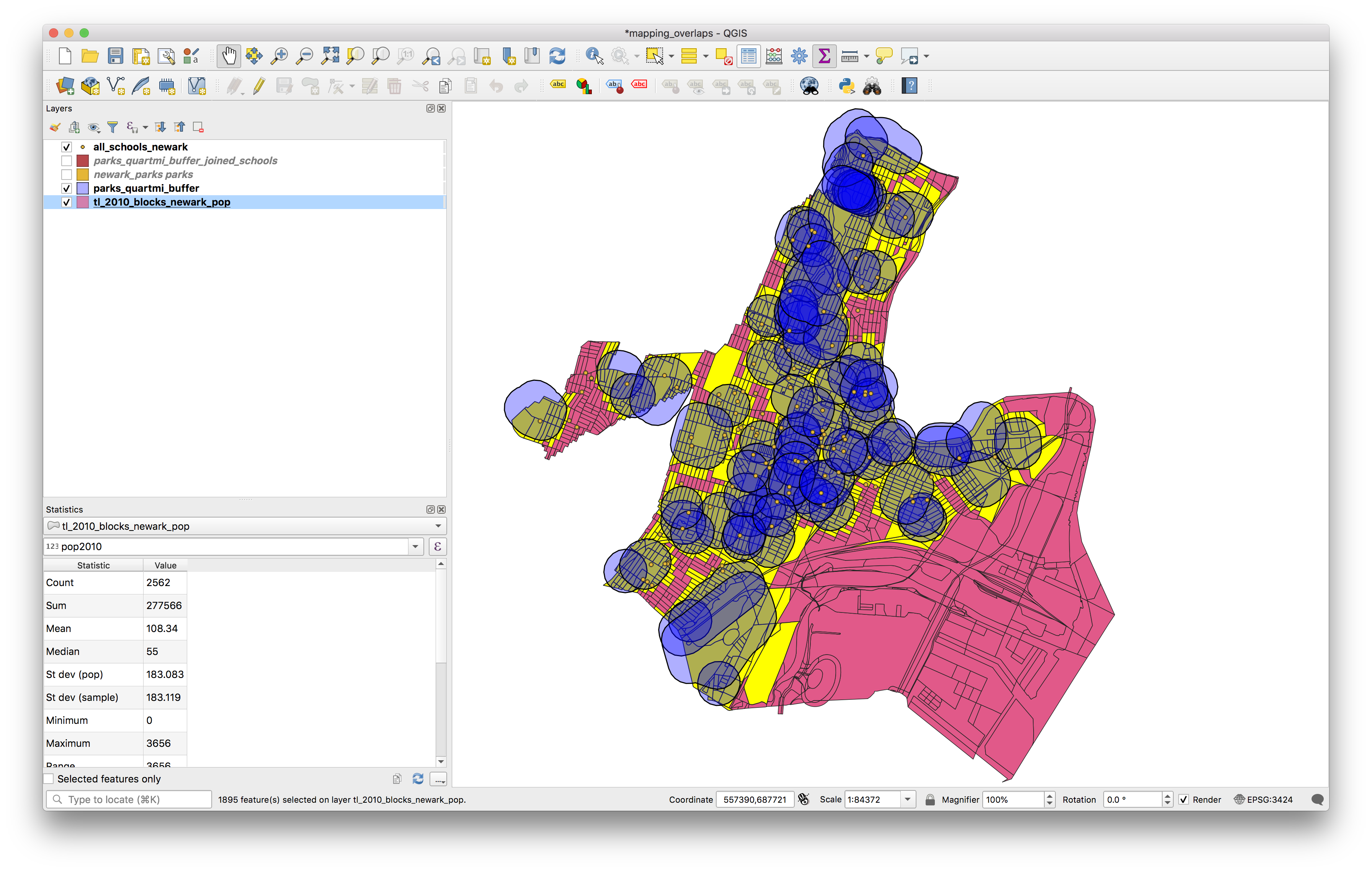
Now un-check the selected features only box to find the total Newark population according to the 2010 census.

Clear the selected features.

Proportional Split Estimation

Now to refine that method we will use a series of geoprocessing steps in a method called proportional split estimation. (For further background on this method, see Schlossberg 2003)

In this method we will obtain an estimate for the population within 1/4 mile of parks, that takes into account the fact that for many census blocks only a portion of the census block intersects with the buffer around each park.

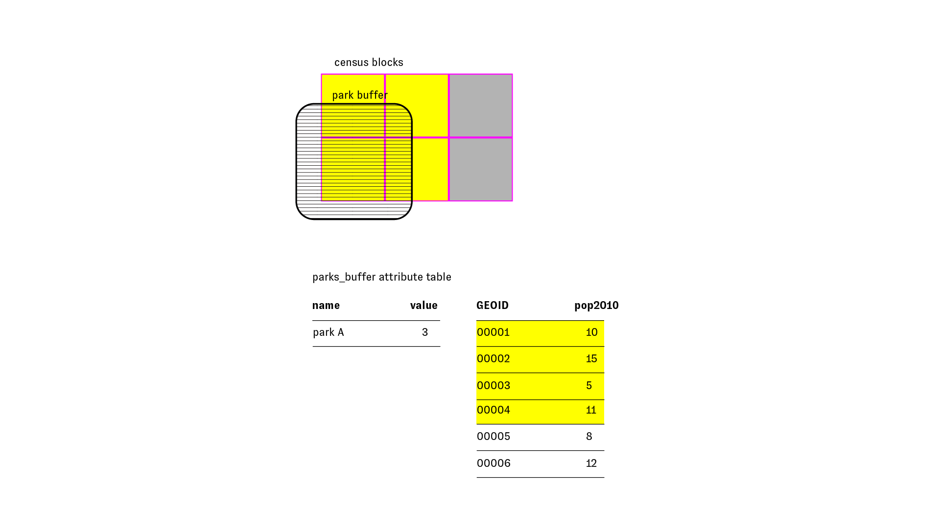
We do this by computing the proportion of the total area of the block that falls within the study area (in our case the buffer). We then multiply this by the total population of the block to obtain an estimate of the population within the study area.

The diagram below illustrates:

This relies on one key assumption that people are spread evenly across the whole census block (which, of course, in reality they are not). It is crucial to keep in mind that this is just an estimate. Its a better estimate than the previous method, but nevertheless it is just an estimate.

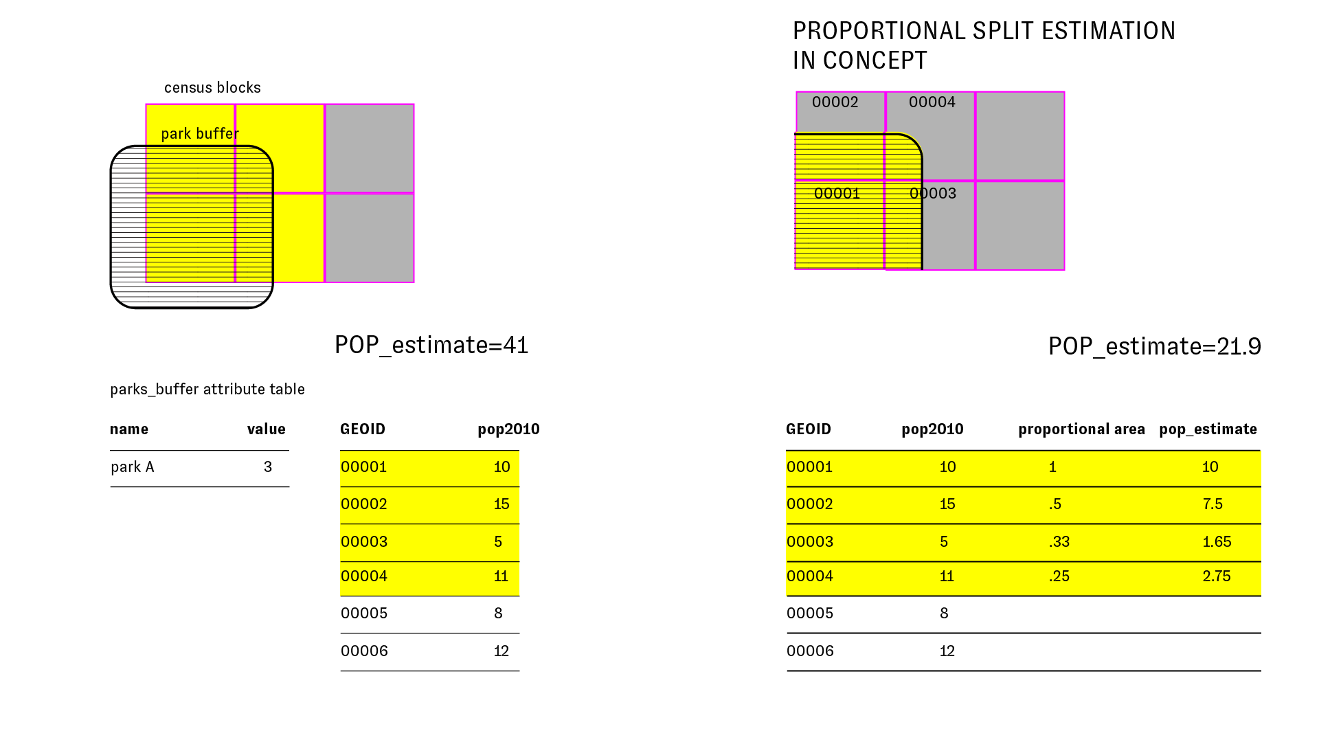
The diagram below explains the proportional split methodology that we will execute in the preceding steps in detail. Please take a close look at this diagram:

Now to implement the above method in QGIS.

First we’ll calculate a new field in the Newark census blocks data layer which will contains the total area of each census block.

Open the attribute table for the Newark census blocks data layer. Open the field calculator (looks like an abacus).

When the field calculator dialog box opens make the following selections and then click OK.

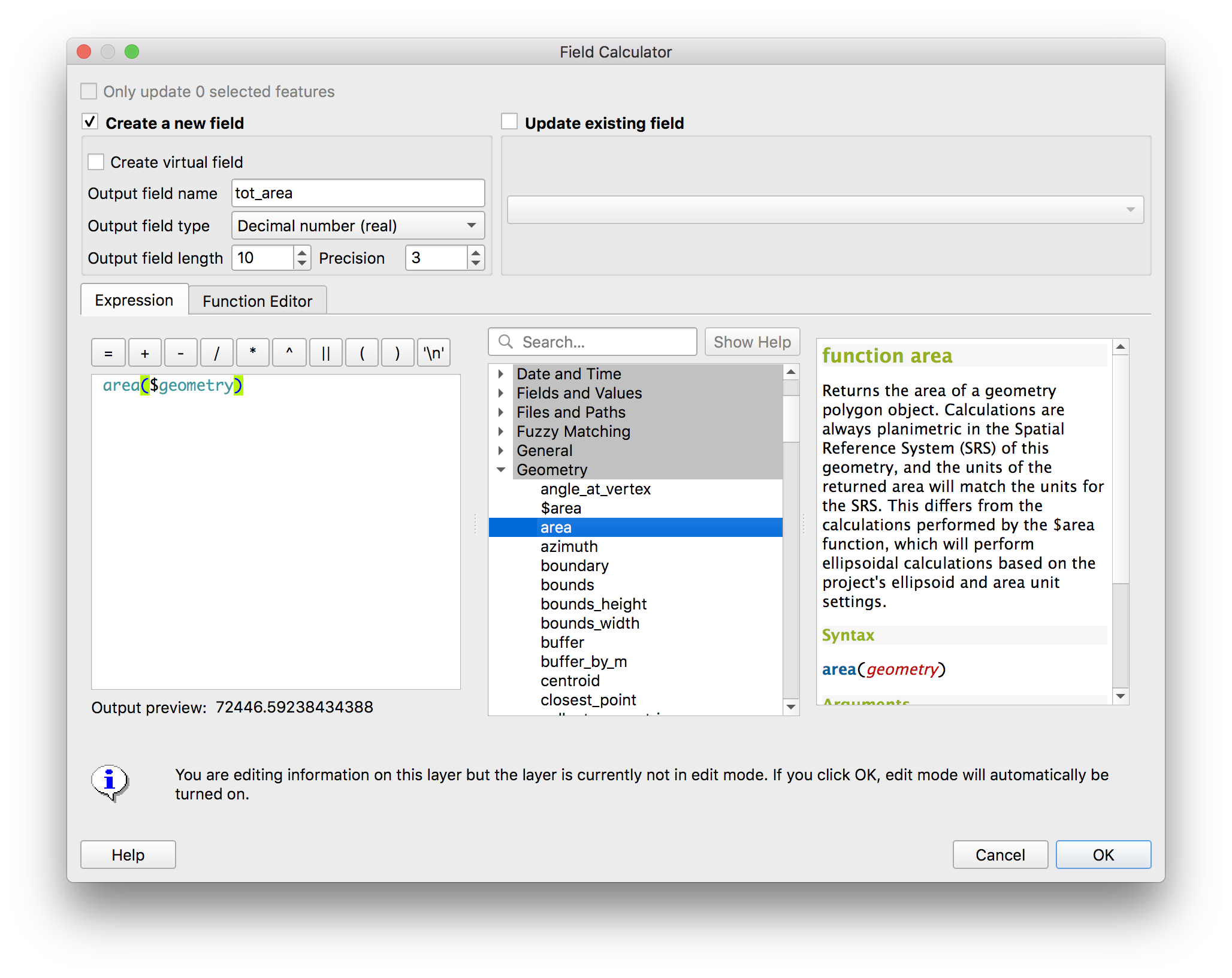
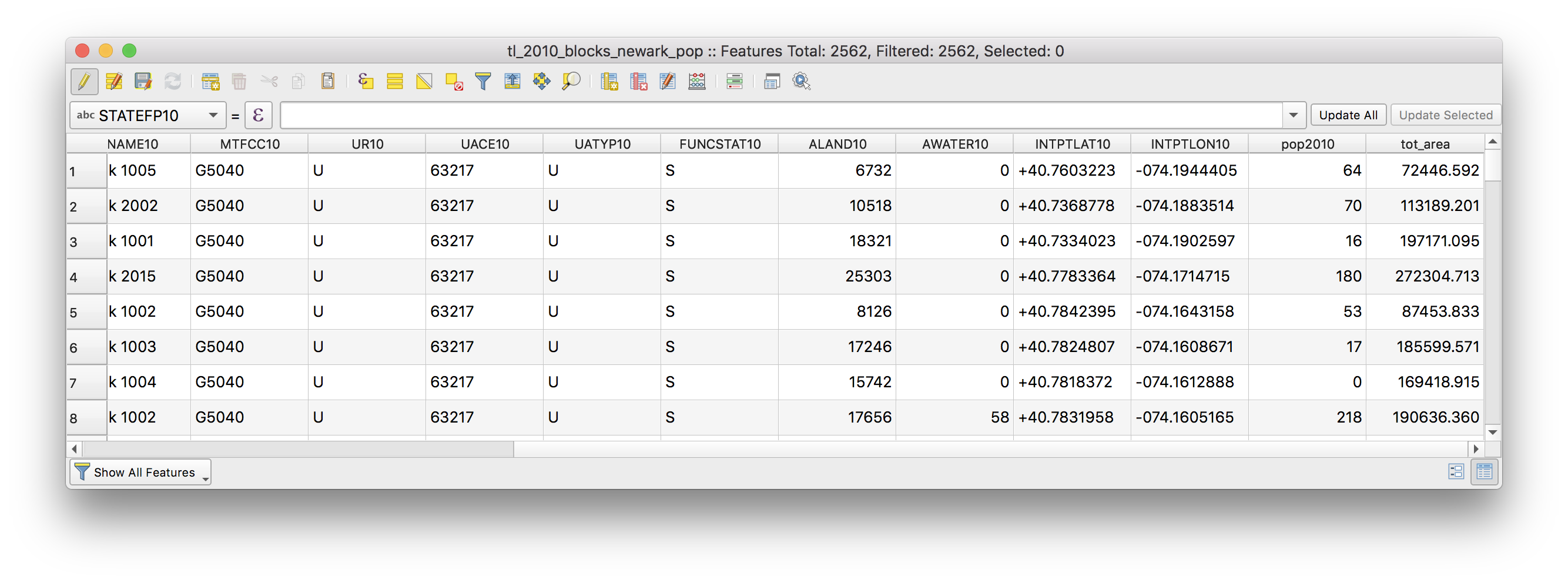
There should be a new field in the attribute table called tot_area with the area for each census block.
What are the units for the area that was calculated?(hint: it is the units that are used by the coordinate reference system of the data layer).

Dissolve

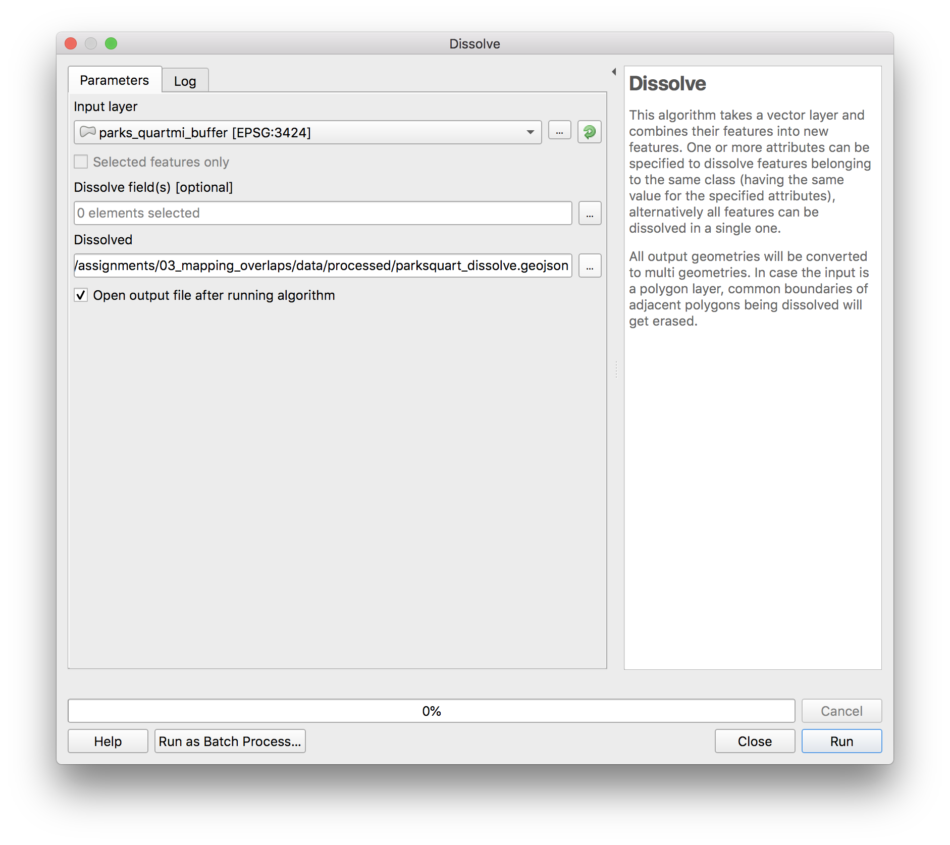
Next because we want the total Newark population that lives within 1/4 mile of any park we will dissolve the park buffers so that there are no longer any areas of overlap. note: If we were instead interested in the population within 1/4 mile of each park we would not do this.

Open vector>geoprocessing>dissolve. In the dissolve menu which will appear select parks_quartmi_buffer.geojson as the input layer. Do not select any dissolve field – we are trying to get a single multi-part polygon for all of the parks buffers. If we instead wanted to dissolve all of the buffers according to some field in the attribute table then we would select that field for the dissolve field. Save the new feature class in the process folder as parksquart_dissolve.geojson

Intersection

Now we are ready to compute the intersection of the polygon representing all of the areas within 1/4 mile of parks in Newark and the census blocks. Computing the intersection of these layers will give us just those areas of each census block that falls within 1/4 mile of a park.

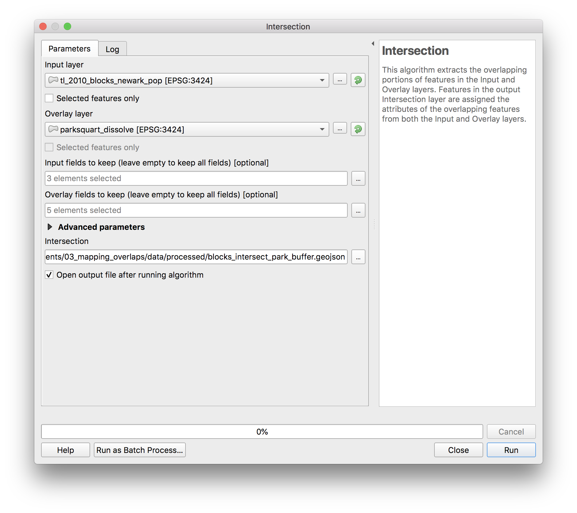
Open Vector>geoprocessing>intersection. In the menu that opens select the Newark census blocks as the input layer and the dissolved buffers around each park as the overlay layer.

To have a more manageable attribute table in the output feature class, use the ... button to keep only the necessary fields from the input layer (left) and from the overlay layer (right):

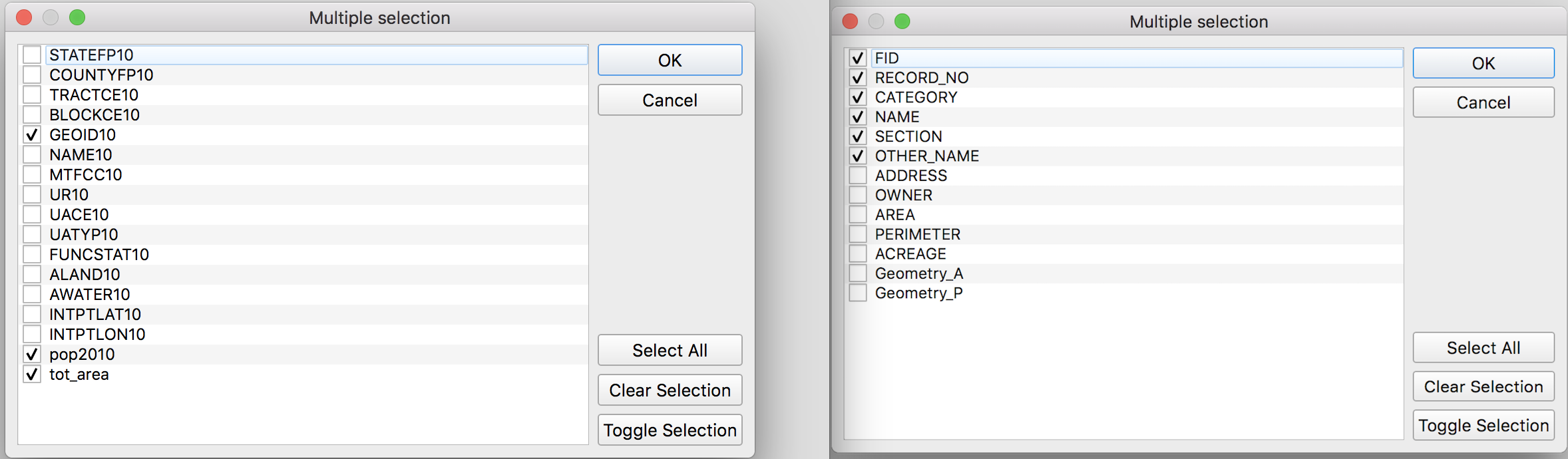
Save the output feature class in the process folder as blocks_intersect_park_buffer.geojson

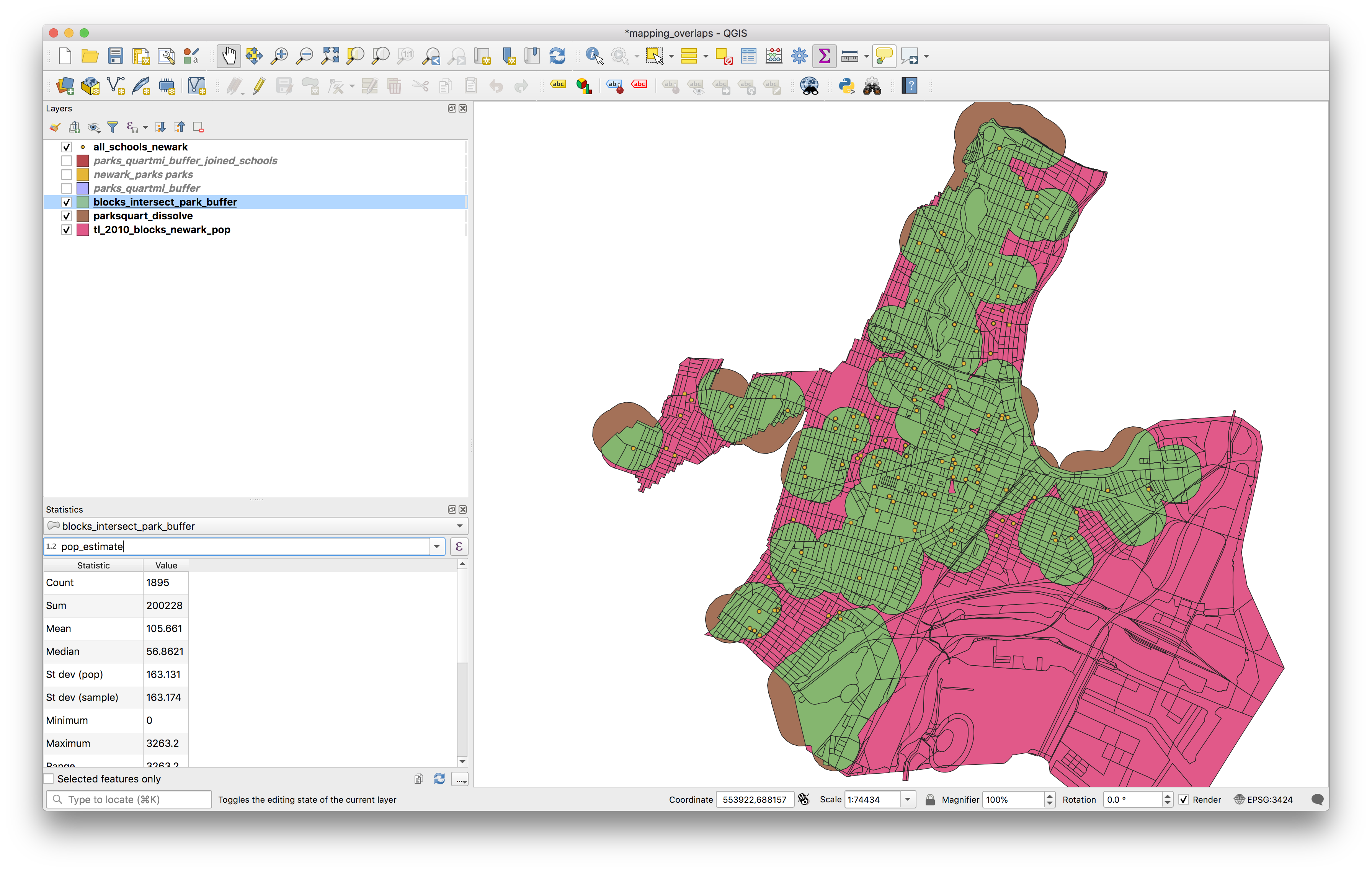
The results should look like this layer shown in green here:

Open the attribute table for the new feature class. It should look like this

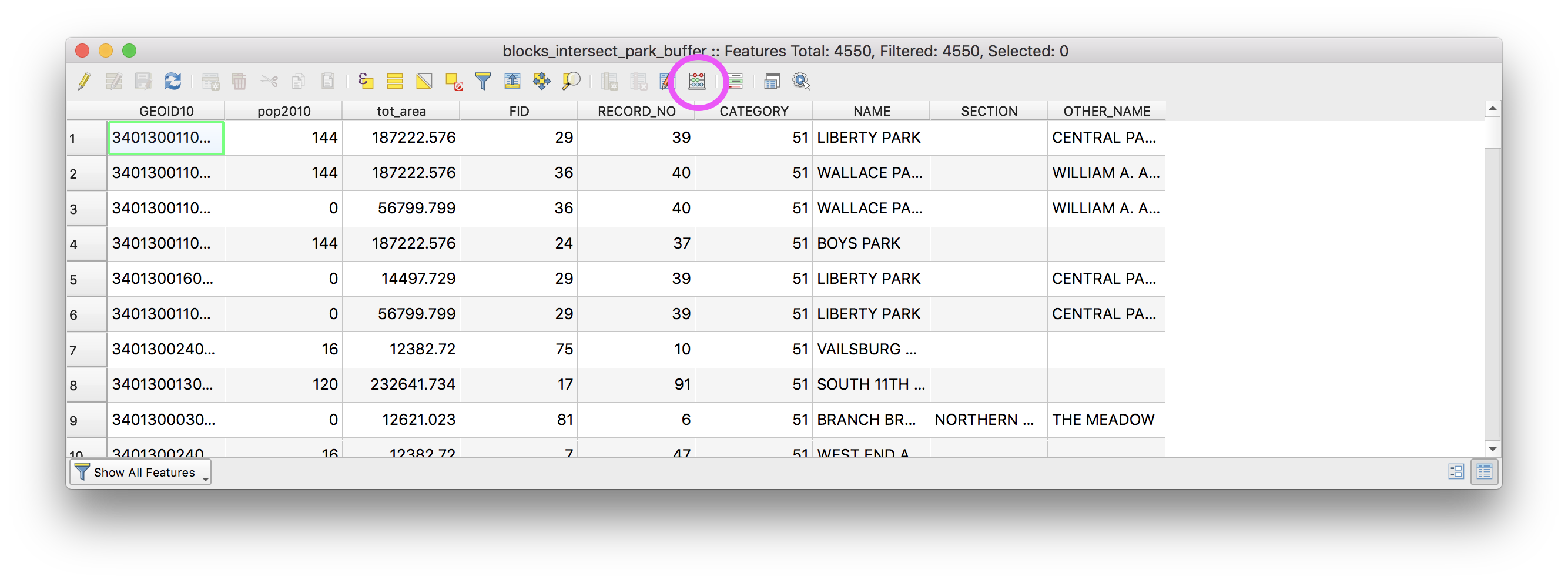
Now we will calculate what proportion of the original block area the new area of each block is. Open the field calculator (circled above) and make the following selections then click OK.

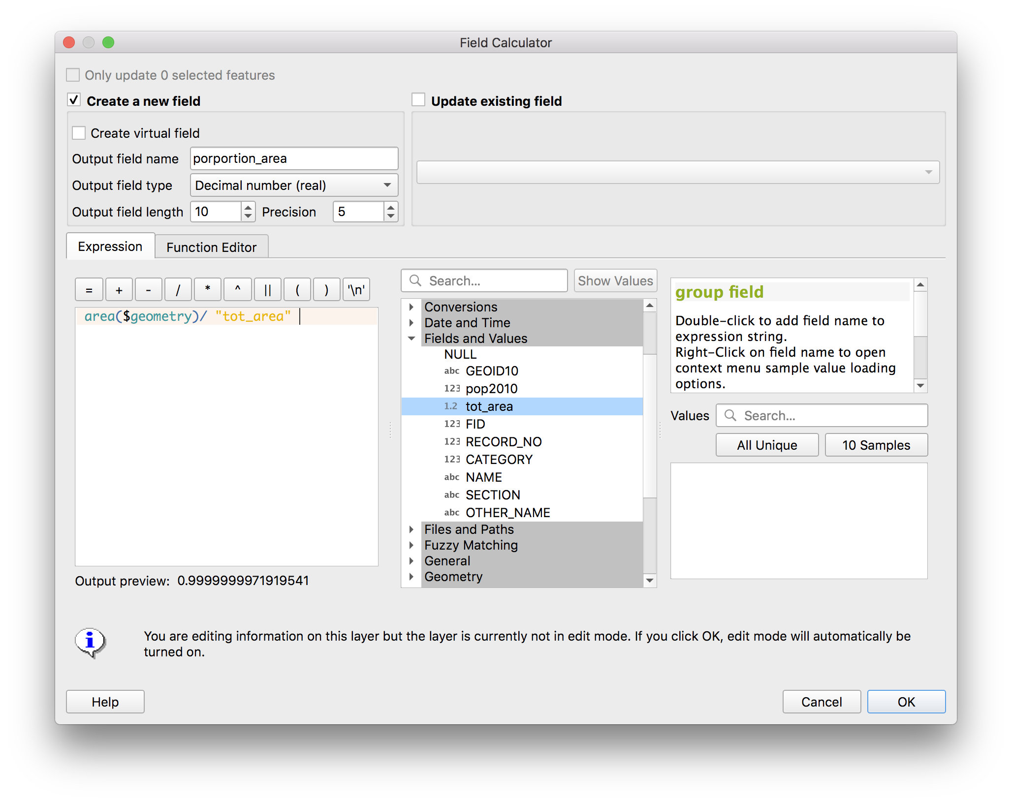
A new field should be added to the attribute table called “proportion_area”. Now we will use this to estimate the proportion of the population of each full census block that lives within each census block portion.

Open the field calculator again and make the following selections, then click OK.

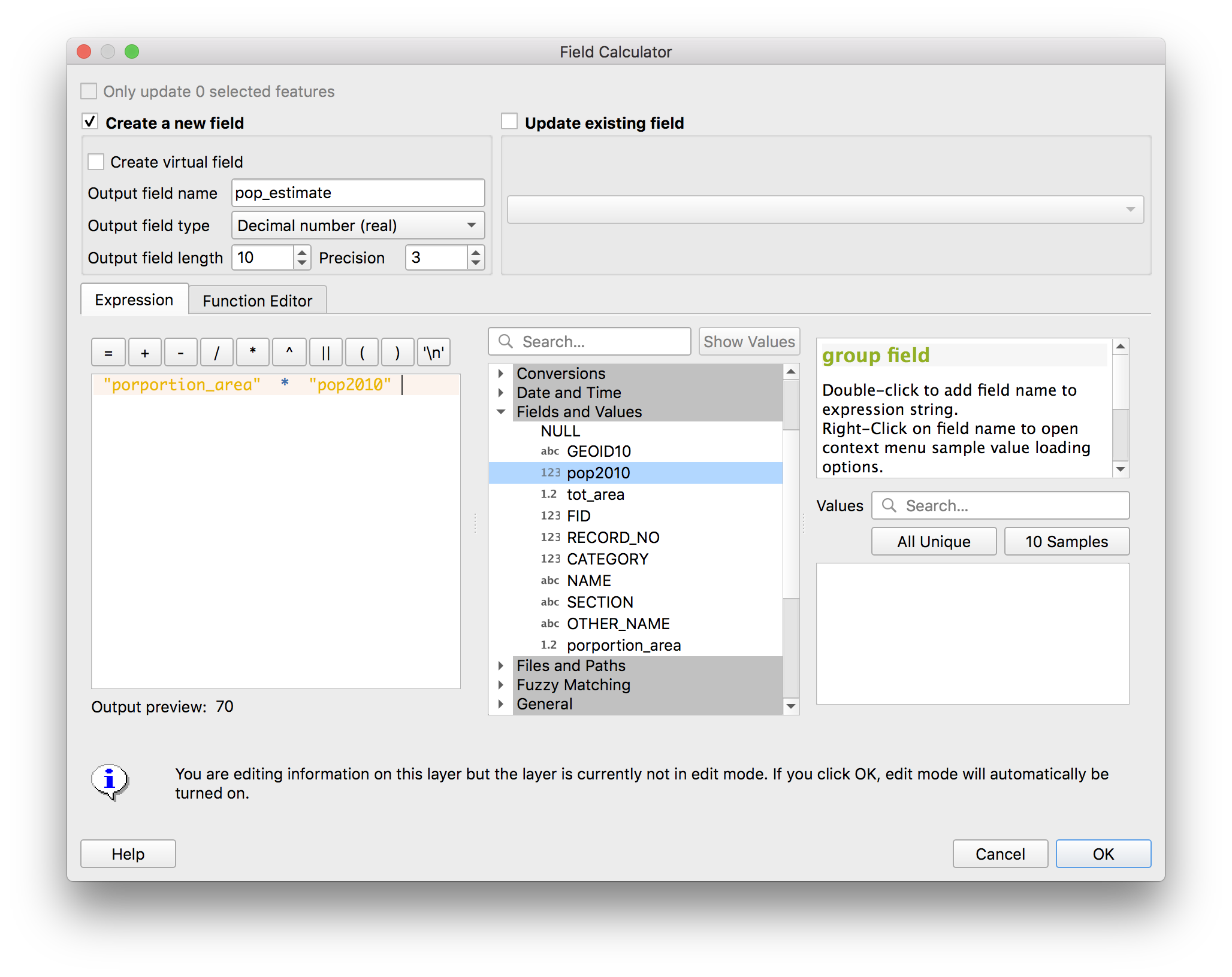
The attribute table should again have a new field (“pop_estimate”) added:

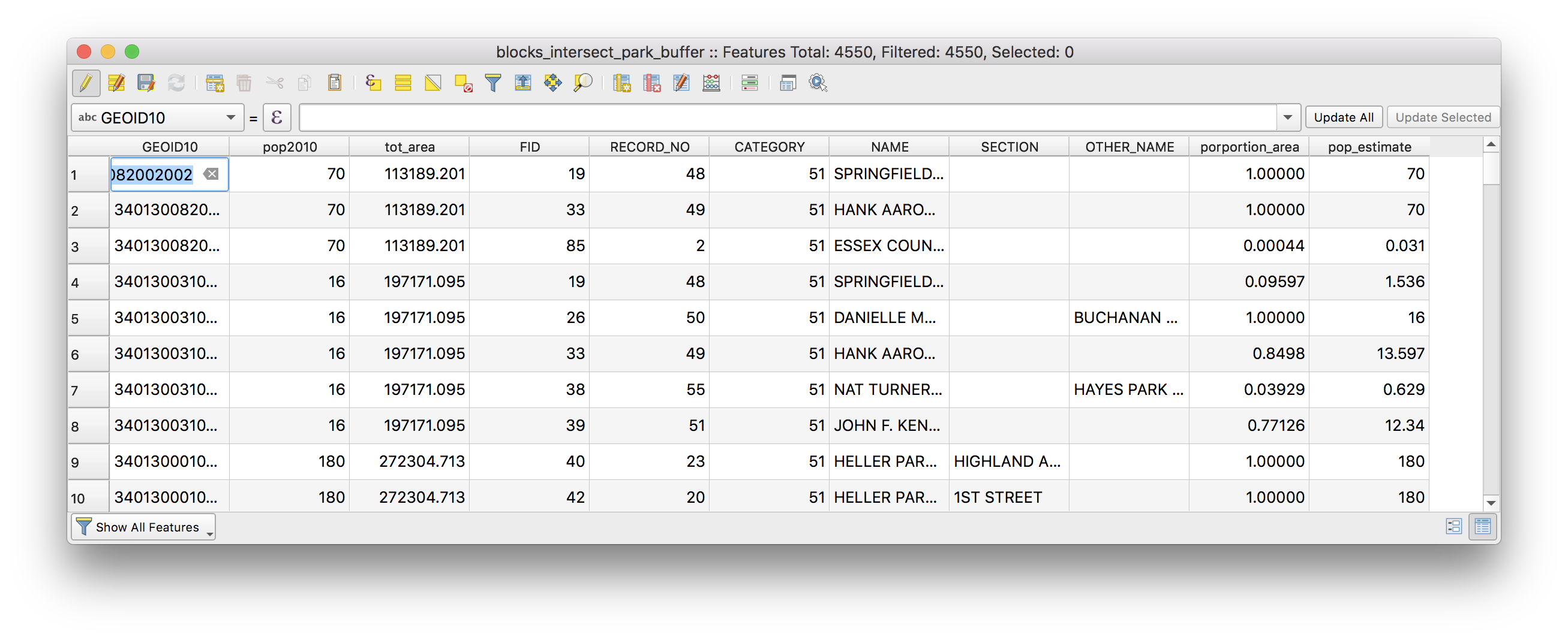
Now again use the show statistical summary tool to find the total for the “pop_estimate” field. What proportion of Newark’s population lives within 1/4 mile of a park using a proportional split estimate?

Geoprocessing in concept

Once you have completed the above please download this PDF with exercises to help you solidify your understanding of geoprocessing operations. In particular the PDF asks you to reason through the impact of each geoprocessing operation on the geometry and/or attribute table. Please annotate/draw on the PDF answering the questions on each page. (Note you must be logged in to your NJIT email to access the PDF)